Tracking hummingbirds at the feeder

Reading time: 8 minutes

Series overview

This is the first post in our deep-dive series on the data from our hummingbird detection. We’ll cover a few different things:

1. Data cleaning (this post)
2. Bird sizes
3. Migration behaviour and weather effects
4. Territorial rufous!

All the data analyzed here was collected in 2021. In the future, we may be able to learn more by comparing across different years. We have images from the hummingbird feeder, and micro-climate data collected from the weather station.

Background

There are two species of hummingbirds found near Galiano: the green Anna’s Hummingbird and the orange Rufous Hummingbird. ID images from allaboutbirds.org.

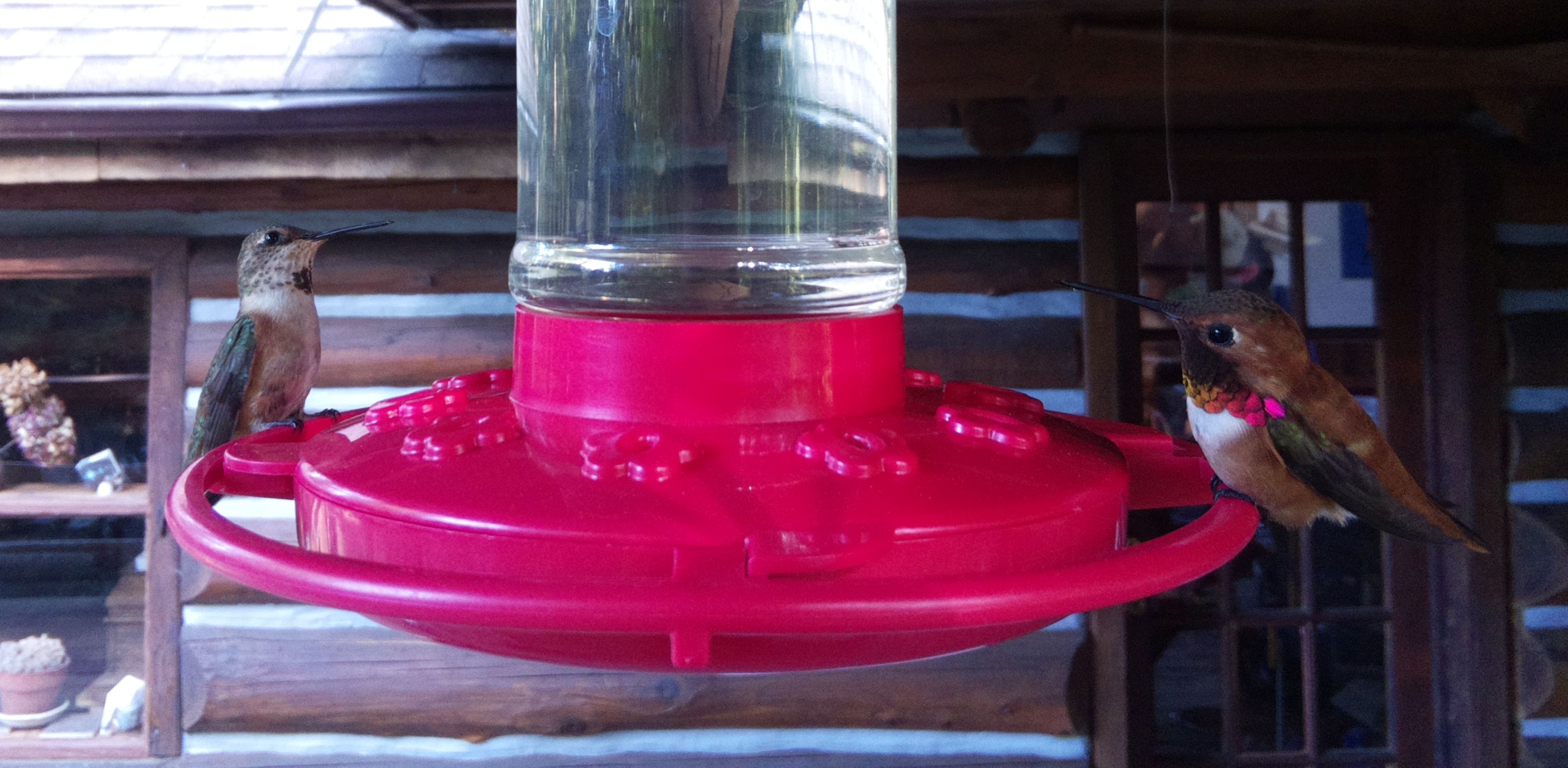
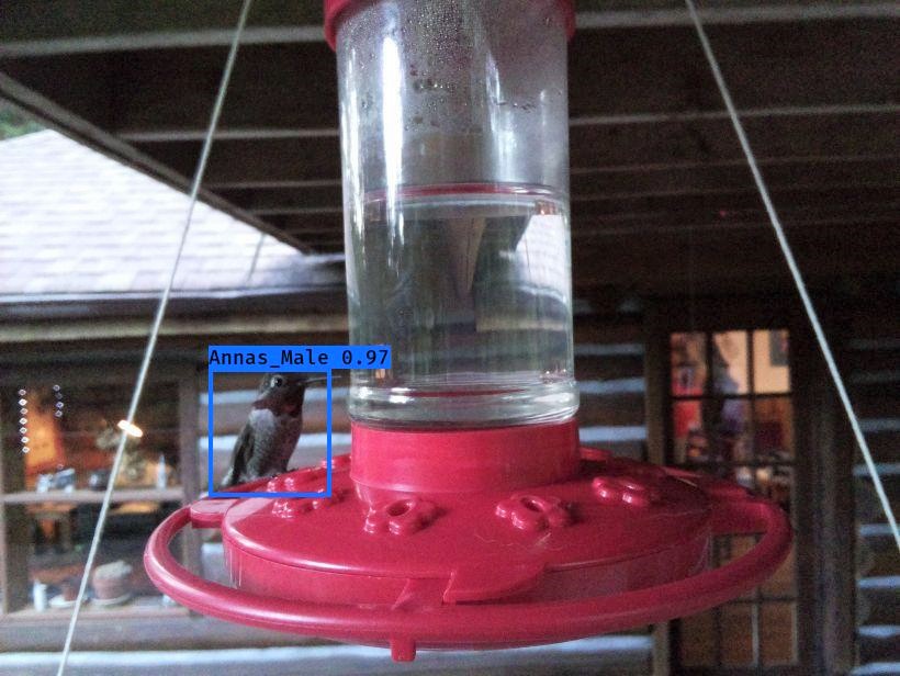
We set up a camera to capture these feathery fellows visiting our hummingbird feeder.

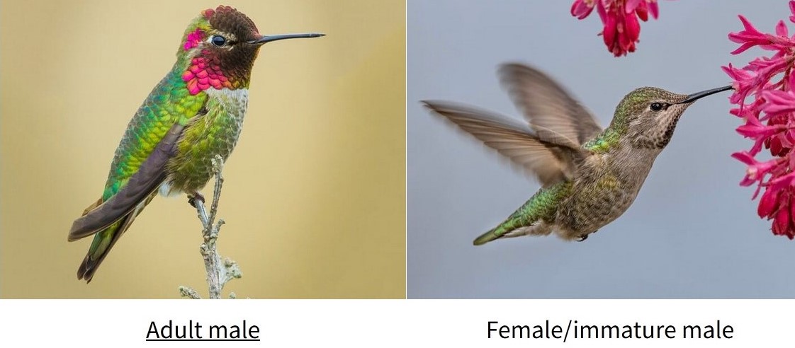
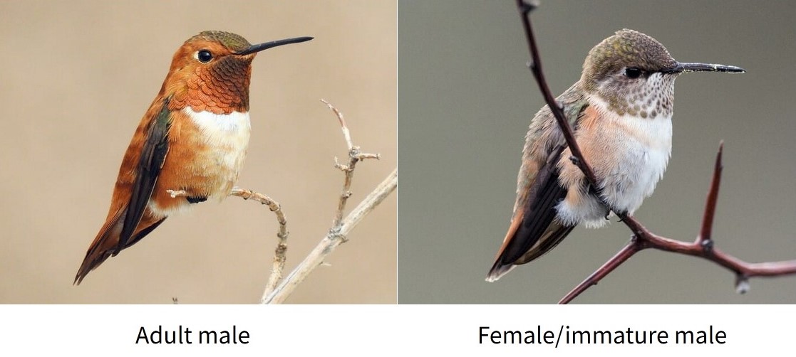
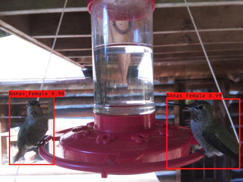
A Female Anna’s (left) and Male Rufus (right) at our feeder

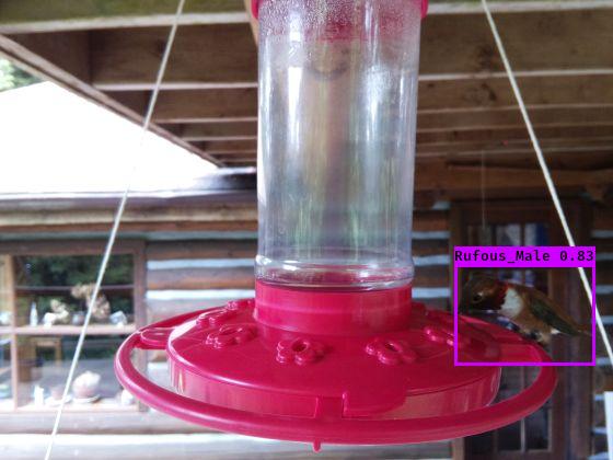
We trained a classifier to detect who’s who….

And we’re even able to keep track of when the feeder needs a refill!

Setup

Lets dive in to some of the data we’ve collected!

We’ll read in and prepare our data: the classifier output as well as bounding boxes of detected birds.

library(tidyverse)
library(lubridate)
library(patchwork)
library(ggpubr)

# classifier labels
classes = c('Rufous_Male', 'Annas_Male', 'Person', 'Annas_Female', 'Rufous_Female')

# read in bird detection data, and do some basic data cleaning
bird <- read_csv('2021_reprocessed_hummers_combo_2023.csv') %>% 
  # lookup labels
  mutate(class = classes[label + 1]) %>%
  # put columns into tidy format
  separate(class, into=c('Species', 'Sex'), sep='_') %>%
  separate(image, into=c('Date', 'image'), sep="_", remove = F) %>%
  separate(image, into=c('hhmm'), sep=".jpg", extra = 'drop') %>%
  # clean up timestamps
  mutate(Timestamp = ymd_hm(paste(Date, hhmm))) %>%
  # remove people
  filter(label != 2) %>%
  # change column types, correct for variable image size
  mutate(Date=ymd(Date),
         Month=factor(month(Date, label = T)),
         Hour=hour(Timestamp),
         Species = ordered(Species),
         Sex = factor(Sex),
         MergeTime = floor_date(Timestamp, 'hour'),
         xmid = (xmax+xmin)/2, 
         ymid = (ymax+ymin)/2
  ) 

The bird detector gives us the the bounding box of each bird in an image, and the predicted sex and species of the bird. Note that because it’s hard to distinguish female birds from the immature males, the “female” class label encompasses both of these. Lets take a peek at the data.

knitr::kable(head(bird))

Date	hhmm	xmin	ymin	xmax	ymax	label	confidence	x_size	y_size	Mo	OK	Species	Sex	Timestamp	Month	Hour	MergeTime	xmid	ymid
2021-04-20	1651	154	365	331	514	0	0.8494033	820	616	04	1	Rufous	Male	2021-04-20 16:51:00	Apr	16	2021-04-20 16:00:00	242.5	439.5
2021-04-20	1706	200	382	406	478	0	0.8925107	820	616	04	1	Rufous	Male	2021-04-20 17:06:00	Apr	17	2021-04-20 17:00:00	303.0	430.0
2021-04-20	1718	634	401	814	552	0	0.9755894	820	616	04	1	Rufous	Male	2021-04-20 17:18:00	Apr	17	2021-04-20 17:00:00	724.0	476.5
2021-04-20	1914	164	389	368	507	0	0.6146710	820	616	04	1	Rufous	Male	2021-04-20 19:14:00	Apr	19	2021-04-20 19:00:00	266.0	448.0
2021-04-20	1925	196	389	408	472	0	0.9455948	820	616	04	1	Rufous	Male	2021-04-20 19:25:00	Apr	19	2021-04-20 19:00:00	302.0	430.5
2021-04-20	1942	177	402	378	539	0	0.9968680	820	616	04	1	Rufous	Male	2021-04-20 19:42:00	Apr	19	2021-04-20 19:00:00	277.5	470.5

Number of birds by species

Our bird detector ID’d lots of visitors! Each ID represents a bird captured in an image, and not necessarily an individual. The images are captured once every minute, so if for example a single bird sat at the feeder for two minutes in a row, it would get counted twice. There may be multiple birds in a single image.

n_table <- bird %>%
  group_by(Species, Sex) %>%
  summarise('Number of ids' = n(), .groups = 'keep')

n_table %>%
  kableExtra::kbl() %>%
  kableExtra::kable_styling(full_width = F)

Species	Sex	Number of ids
Annas	Female	4127
Annas	Male	1792
Rufous	Female	11720
Rufous	Male	1081

🧠 Observation

There are more Rufouses than Annas, and many more females + immature males than mature males captured in our images.

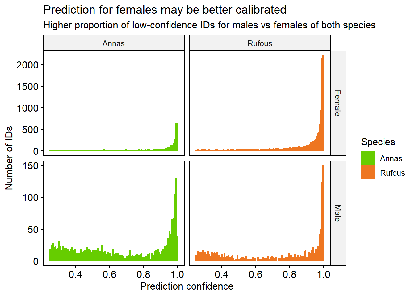
Classifier confidence

Each bird ID is made by picking the the most likely label, based on the prediction probability. Sometimes, the classifier isn’t as confident as others. For example, it may be harder to identify a bird that is facing away from the camera. We can plot the confidences, and see which birds are the hardest to label.

bird %>%
  gghistogram(x = 'confidence', fill = 'Species', color='Species', bins=100,
              facet.by = c('Sex','Species'), scales = 'free_y', alpha=1, position='stack') +
  labs(title = 'Prediction for females may be better calibrated',
       subtitle = 'Higher proportion of low-confidence IDs for males vs females of both species', 
       x = 'Prediction confidence', y = 'Number of IDs') + 
  theme(legend.position = 'right') + 
  scale_fill_manual(values=c('chartreuse3', 'chocolate2')) + 
  scale_colour_manual(values=c('chartreuse3', 'chocolate2'))

There is almost certainly some mistakes in our classifier, including false positives (non-birds labeled as birds) and false negatives (birds that are missed)

To help make sure we’re only considering high-quality calls, we’ll pick a confidence threshold of 0.7 and only analyse the IDs above that level.

🧠 Observation

For both species, mature male birds are slightly harder to identify with high confidence than female + immature male. This may be because there are fewer of them.

Filtering for high-confidence IDs

We manually looked at the images, and found that that almost all the Rufouses after September 1st are false positives, so we’ll remove these observations. Also, since we have few IDs in October compared to other months, we will drop this month from our data. Then, we’ll filter to only retain the high-confidence (> 0.7 prediction probability) bird IDs

table(bird$Month) %>%
  t() %>%
  kableExtra::kbl() %>%
  kableExtra::kable_styling(full_width = F)

Apr	May	Jun	Jul	Aug	Sep	Oct
1125	4701	6063	2724	2164	1875	68

bird <- bird %>%
  filter(!(Timestamp >= ymd('2021-09-01') & Species =='Rufous')) %>%
  filter(Timestamp < ymd('2021-10-01')) %>%
  filter(confidence > 0.7)

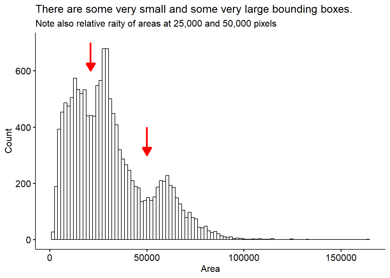
Lastly, we’ll sanity check the bounding boxes for their size.

bird <- bird %>%
  mutate(
    Height = ymax-ymin, 
    Width = xmax-xmin, 
    Area = Height * Width
  )

bird %>% 
  gghistogram(x="Area", bins = 100) + 
  annotate("segment", x = 21000, xend = 21000, y = 700, yend = 600, size = 1.2,
           colour = "red", arrow = arrow(type='closed', length=unit(0.04, 'npc')))  + 
  annotate("segment", x = 50000, xend = 50000, y = 400, yend = 300, size = 1.2,
           colour = "red", arrow = arrow(type='closed', length=unit(0.04, 'npc')))  + 
  labs(title = 'There are some very small and some very large bounding boxes.',
       subtitle = "Note also relative raity of areas at 25,000 and 50,000 pixels", y = 'Count')

This distribution more or less makes sense, we see some very small bounding boxes which may be mis-calls or birds who are only half in the image. There are also some cases where a bird is partially obscured because it’s sitting behind the feeder. There are some very large bounding boxes also. I’m not sure exactly whether these are real, giant humming birds, or some kind of error.

Lets see if looking at the bird position with respect to the feeder helps sort this out.

Batch correction and normalization

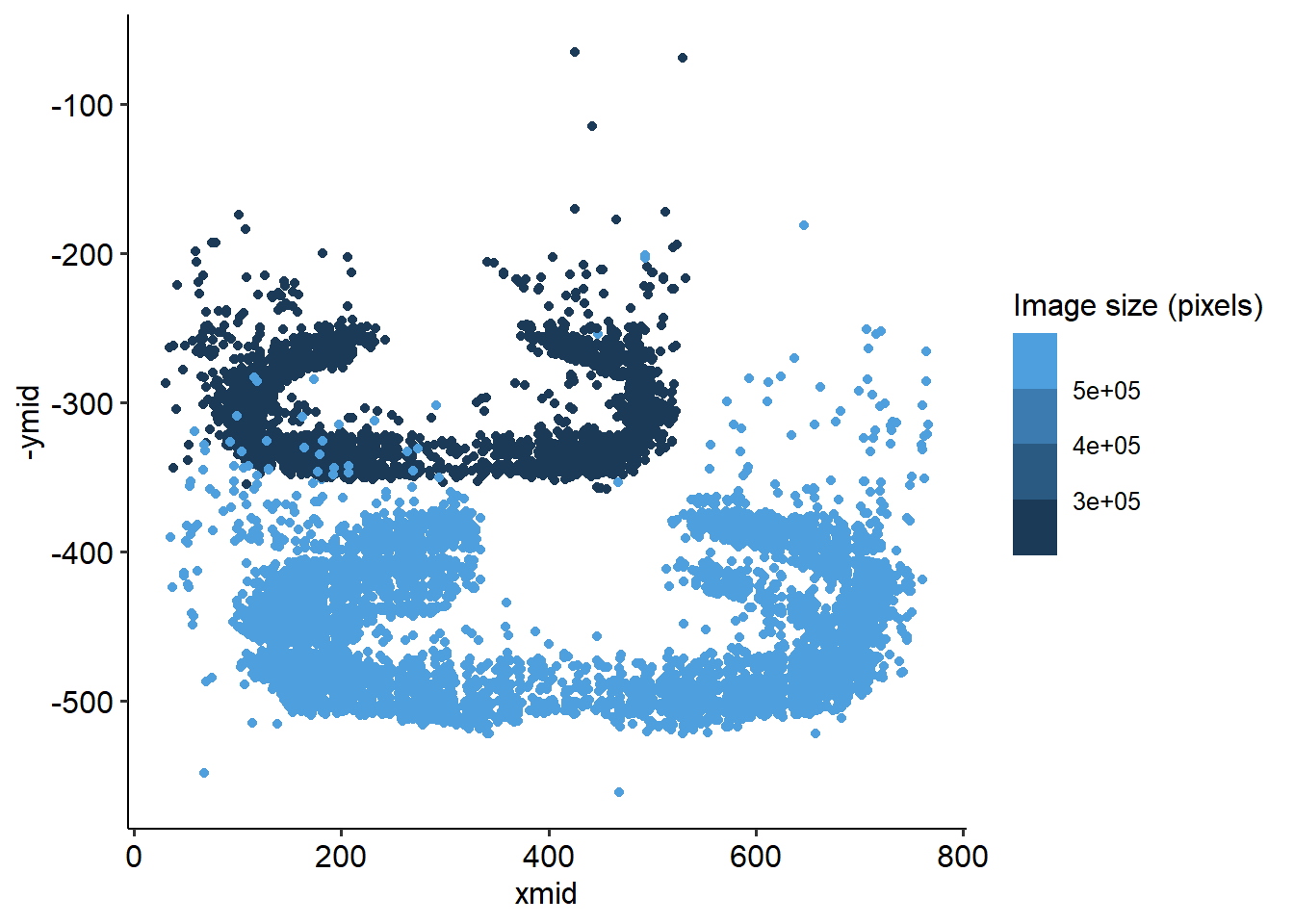
We can plot the location of where each bird sits, with the proxy that a birds will be located at the center of its bounding box (indicated by xmid and ymid). The birds appear to mostly sit in a circle, around the rim of the feeder. This gives the best access to the sugar water.

bird %>% ggplot(aes(x = xmid, y = -ymid, colour=y_size * x_size)) +
  geom_point() +
  theme_pubr() + 
  labs(colour = 'Image size (pixels)') + 
  scale_colour_binned(n.breaks=3) + 
  theme(legend.position = 'right', legend.direction = 'vertical') 

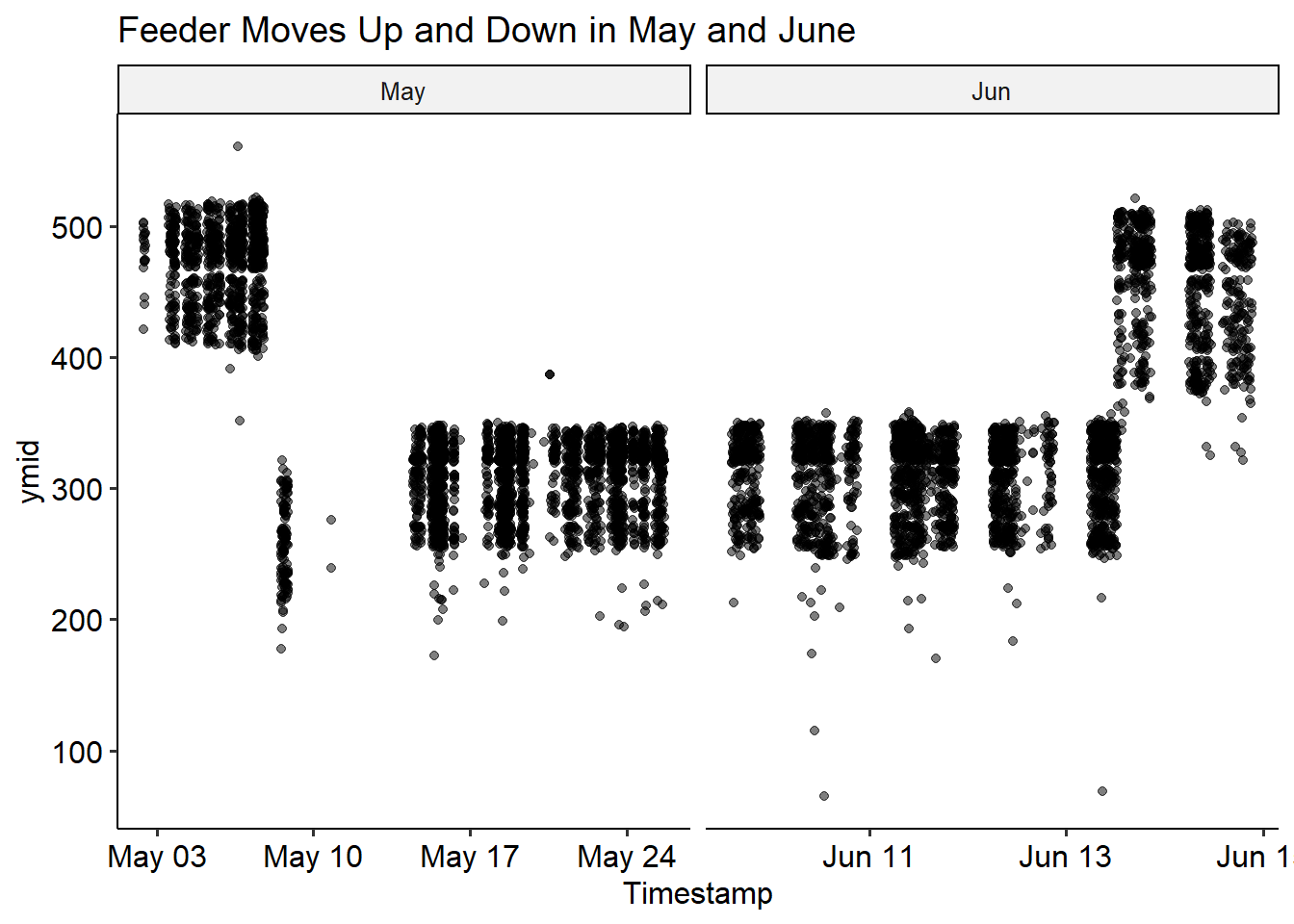
However, it looks like there are at least 2 distinct positions that the feeder was in over the summer. We’ll try to do batch correction for this, by assigning a batch number to each position, and subtract the average from the x and y direction. I think we can reasonably split the changes in position (the batches) simply by the date. This is easy to see in the ymid variable - the feeder moves twice in May, and once in June.

bird %>% 
  mutate(Month = month(Date, label=T)) %>%
  filter(Date>'2021-05-01' & Date<'2021-06-15') %>%
  ggplot(aes(x=Timestamp, y = ymid))+ 
  geom_jitter(alpha = 0.5) + 
  facet_wrap("~Month", scales = 'free_x') + 
  theme_pubr() + 
  labs(title = 'Feeder Moves Up and Down in May and June')

Lets split these into batches for correction.

bird$Batch <- 1
bird$Batch <- ifelse(bird$Timestamp > ymd_hms('2021-05-08 00:00:00'),2,bird$Batch)
bird$Batch <- ifelse(bird$Timestamp > ymd_hms('2021-05-11 00:00:00'),3,bird$Batch)
bird$Batch <- ifelse(bird$Timestamp > ymd_hms('2021-06-13 12:20:00'),4,bird$Batch)
bird$Batch <- factor(bird$Batch)

We can check it went as expected by recolouring the previous plot by batch

bird %>% 
  mutate(Month = month(Date, label=T)) %>%
  mutate(xmid = (xmax+xmin)/2, ymid = (ymax+ymin)/2) %>% 
  filter(Date>'2021-05-01' & Date<'2021-06-15') %>%
  ggplot(aes(x=Timestamp, y = ymid, color=Batch))+ 
  geom_point(alpha = 0.5) + 
  facet_wrap("~Month", scales = 'free_x') + 
  theme_pubr() + 
  labs(title = 'We can Infer Position Batches Based on When the Feeder Moves',
       colour = 'Batch')

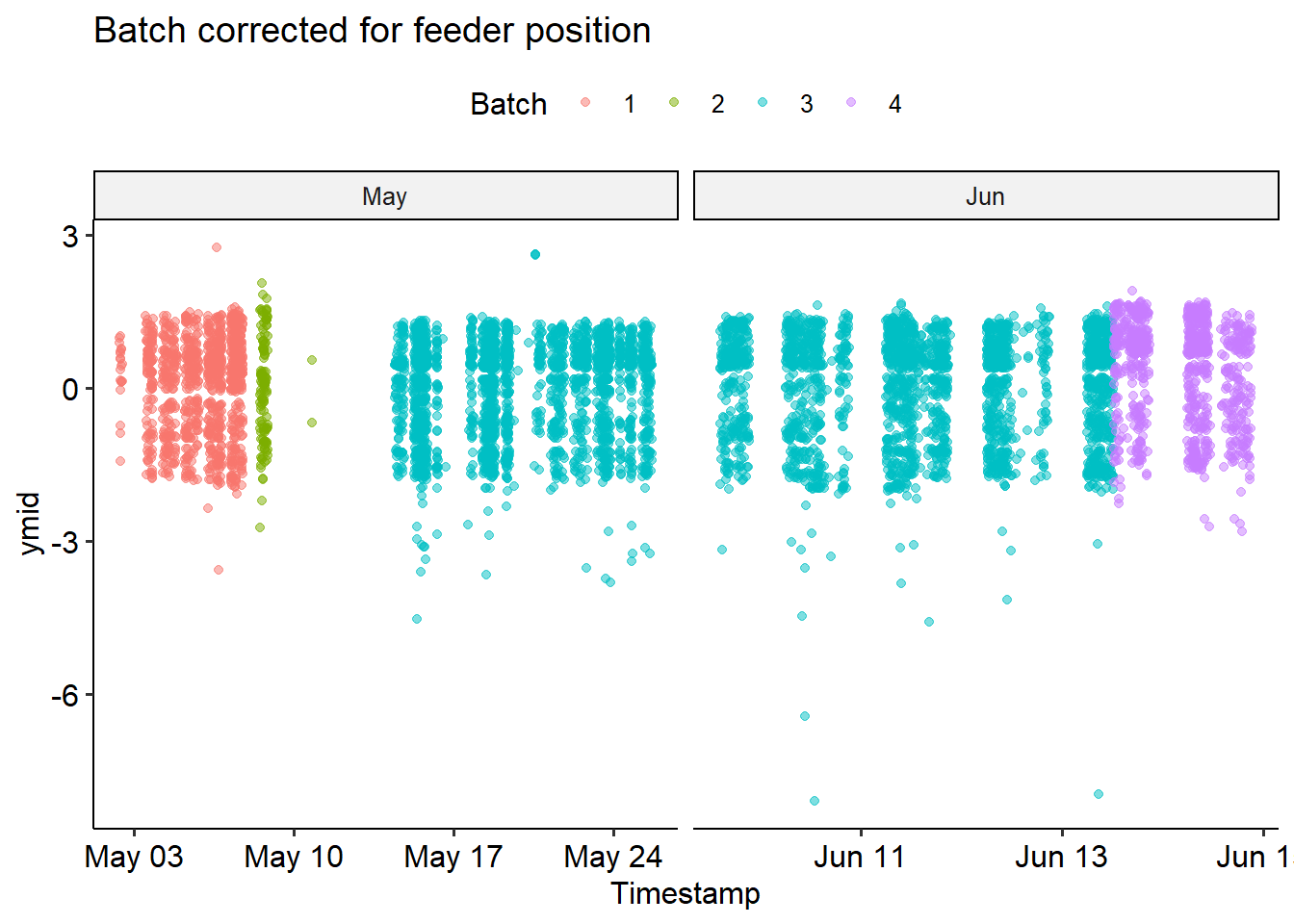
Now we’re ready to correct! We’ll transform all the x- and y- values by centering and scaling each batch. This will yield a new positioning relative to the middle of the feeder; we can no longer interpret this as the pixel index in the image. We’ll normalize the “mid” locations, then add the size of the bounding box back.

bird_scaled <- bird %>% 
  mutate(Month = month(Date, label=T)) %>%
  mutate(Height = ymax-ymin, Width = xmax-xmin) %>%
  group_by(Batch) %>%
  mutate(across(c(Height, Width, xmid, ymid), ~scale(.x))) %>%
  mutate(xmin = xmid - Width/2, xmax = xmid + Width/2, 
         ymin = ymid - Height/2, ymax = ymid + Height/2)

bird_scaled %>% 
  filter(Date>'2021-05-01' & Date<'2021-06-15') %>%
  ggplot(aes(x=Timestamp, y = ymid, color=Batch))+ 
  geom_point(alpha = 0.5) + 
  facet_wrap("~Month", scales = 'free_x') + 
  theme_pubr() + 
  labs(title = 'Batch corrected for feeder position',
       colour = 'Batch')

We can see that the correction didn’t perfectly fix things - but it looks pretty good! From now on, we’ll use the bird_scaled dataframe.

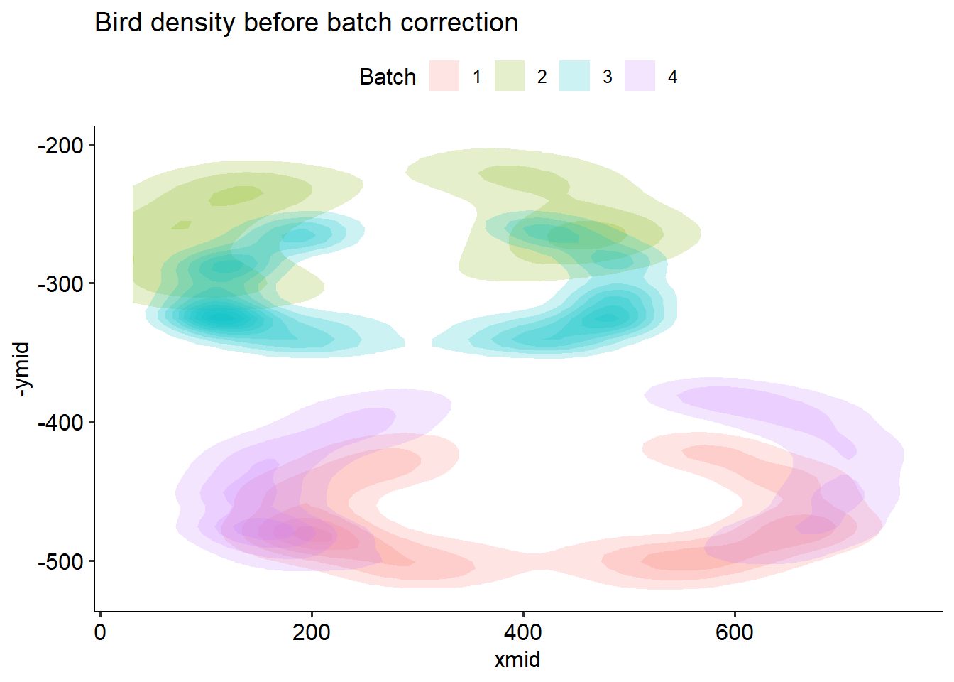
bird %>%
  ggplot(aes(x=xmid, y=-ymid) ) +
  stat_density_2d(aes(fill=Batch), geom = "polygon", alpha=0.2) + 
  theme_pubr() + 
  labs(title = 'Bird density before batch correction', fill = 'Batch')
bird_scaled %>%
  ggplot(aes(x=xmid, y=-ymid) ) +
  stat_density_2d(aes(fill=Batch), geom = "polygon", alpha=0.2) + 
  theme_pubr() + 
  labs(title = 'Bird density after batch correction',fill = 'Batch')

The gap in the middle comes from the water column - we can’t detect birds sitting behind it! Of course, we have to be somewhat careful when converting back to the coordinates of the image. I negate the y coordinates, because they count down from the top of the image.

img <- jpeg::readJPEG('feeder.jpg')

bird_scaled %>%
  ggplot(aes(x=xmid, y = -ymid)) + 
  ylim(-2, 10) + 
  background_image(img) + 
  geom_point(colour = 'lightblue') 

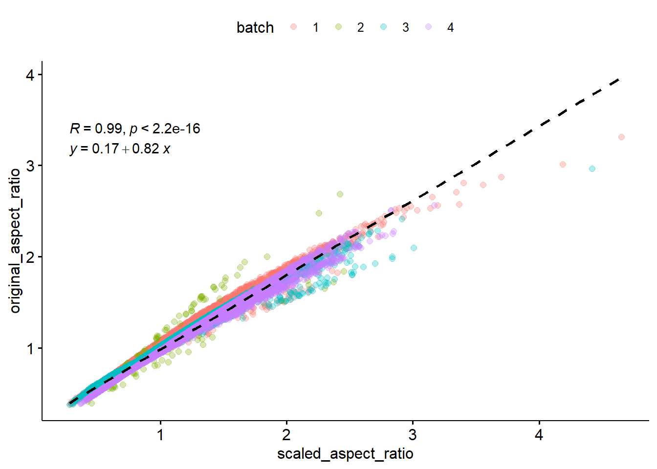
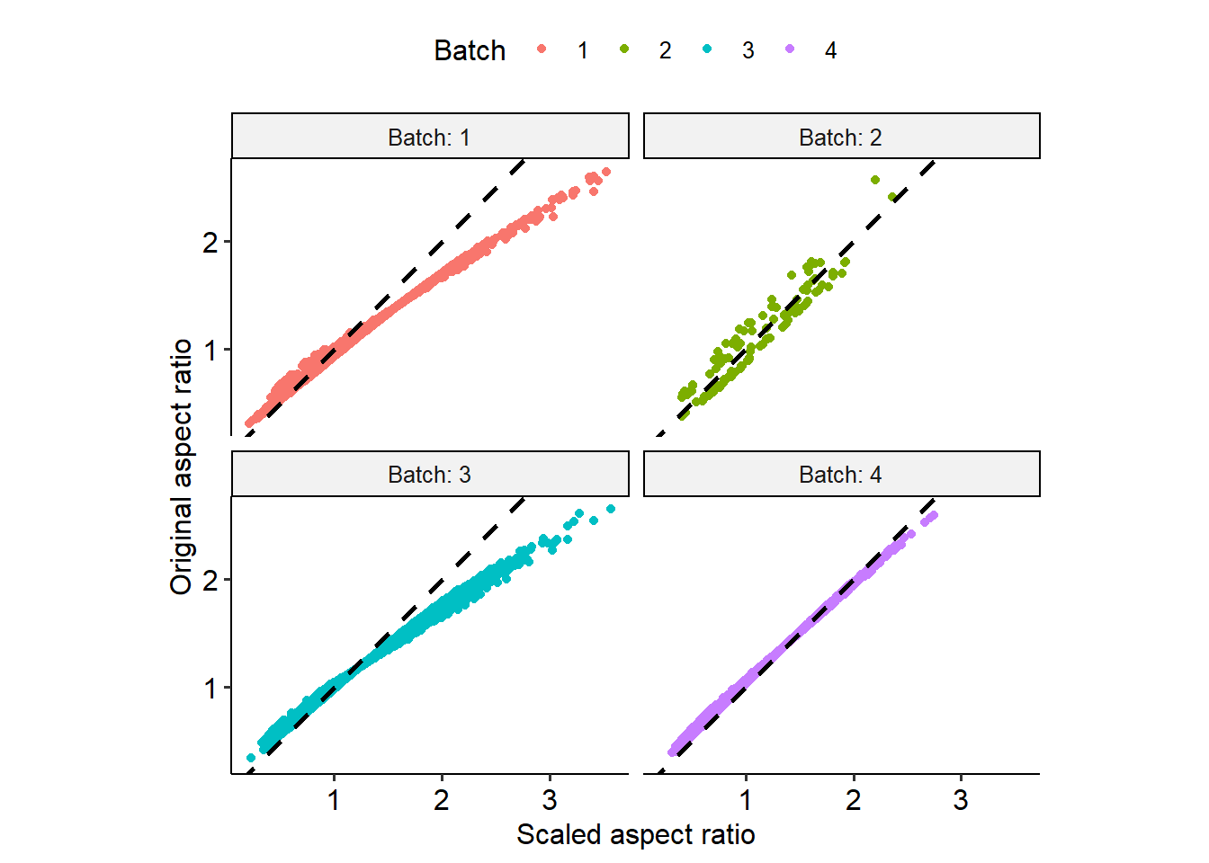
Now we have our corrected bounding boxes! However, since we z-score normalized height and width, there are some negative values. This doesn’t make sense, so we’ll bring these back to the original space by using ungroup to add back the (pooled) mean and standard deviation. At the same time, we can filter out some extreme values (>2 sd from mean).

bird_scaled <- bird %>% 
  mutate(Month = month(Date, label=T)) %>%
  mutate(Height = ymax-ymin, Width = xmax-xmin, 
         original_aspect_ratio = (Width/Height)) %>%
  group_by(Batch) %>%
  mutate(across(c(Height, Width, xmid, ymid), ~scale(.x))) %>%
  filter(abs(Height)<=2) %>%
  filter(abs(Width)<=2) %>%
  ungroup() %>%
  mutate(across(c(Height, Width, xmid, ymid), ~(.x * sd(bird$.x)) + mean(bird$.x))) %>%
  mutate(xmin = xmid - Width/2, xmax = xmid + Width/2, 
         ymin = ymid - Height/2, ymax = ymid + Height/2)

Since we normalized height and width independently, We should check that aspect ratio is preserved.

bird_scaled %>%
  mutate(scaled_aspect_ratio = (Width/Height)) %>%
  ggplot(aes(x= scaled_aspect_ratio, y = original_aspect_ratio, colour = Batch)) +    geom_point() + 
  facet_wrap(~Batch, labeller = label_both) + 
  theme_pubr() + 
  coord_equal() + 
  geom_abline(intercept=0, slope = 1, linetype = 'dashed', linewidth = 1) + 
  labs(x = 'Scaled aspect ratio', y = 'Original aspect ratio', colour = 'Batch')

There are some boxes that may have got warped through the normalization, especially in batches 1 and 3, but for the most part it’s not terribly far off.

bird_scaled %>% 
  gghistogram(x="log2(Width/Height)", bins = 100) + 
  labs(title = 'Bounding box aspect ratios after batch correction',
       subtile = 'Relative rarity of values at 18,000 and 38,000',
       y = 'Count') +
  annotate("segment", x = -0.2, xend = -2, y = 430, yend = 430, size = 1.2,
           colour = "red", arrow = arrow(type='closed', length=unit(0.04, 'npc'))) + annotate('text', label = 'Tall & thin', colour = 'red', x = -1, y = 450) +
  annotate("segment", x = 0.2, xend = 2, y = 430, yend = 430, size = 1.2,
           colour = "red", arrow = arrow(type='closed', length=unit(0.04, 'npc'))) + annotate('text', label = 'Short & wide', colour = 'red', x = 1, y = 450)  + 
  annotate('text', label='Square', x = 0, y = 450, colour = 'red')

🧠 Observation

There are more short and wide bounding boxes than tall and thin ones.

Number of ID’s after filtering

After all this filtering, here’s the final numbers of each class label:

n_table %>% 
  bind_cols(
    bird_scaled %>%
    group_by(Species, Sex) %>%
    summarise(n=n(), .groups = 'keep') %>%
    pull(n)
  ) %>%
  rename(`Before filtering` = `Number of ids`,
         `After filtering` = `...4`) %>%
  kableExtra::kbl() %>%
  kableExtra::kable_styling(full_width = F)

Species	Sex	Before filtering	After filtering
Annas	Female	4127	2924
Annas	Male	1792	833
Rufous	Female	11720	9598
Rufous	Male	1081	634

🧠 Observation

There are more Rufouses than Annas, and many more females than males captured in our images.

Summary

We’ve filtered out low-confidence ID’s and suspicious aspect-ratio bounding boxes. Each row in our dataframe corresponds to a picture of a bird, not necessarily an individual. Female and immature males are not possible to distinguish, they are both classified as females. There are more birds labeled as female than male for both Anna and Rufous. There are more Rufous than Anna. Bounding boxes tend to be short and wide more often than tall and thin.

We’ll save the prepared bird_scaled dataframe for future use.

write.csv(bird_scaled, 'bird_scaled.csv')

Read on to Part 2